VISUAL RECURRENCE ANALYSIS
Recurrence Plots (RPs) were first described by J.P. Eckmann, S. O. Kamphorst and D.Ruelle in "Recurrence plots of dynamical systems" in 1987.
( J.P. Eckmann, S. Oliffson Kamphorst and D.
Ruelle,
Recurrence plots of dynamical systems, 1987,
Europhys. Lett., Vol. 4, No. 9, pp. 973-977 )
RP is a relatively new technique for the
qualitative assessment of time series. With RP, one can
graphically detect hidden patterns and structural changes in data
or see similarities in patterns across the time series under
study.
The fundamental assumption underlying the idea of the recurrence
plots is that an observable time series (a sequence of
observations) is the realization of some dynamical process, the
interaction of the relevant variables over time. For example, the
weather is a highly complex system with a large number of factors
that influence its dynamics, and a sequence of daily temperature
readings could be considered a realization of that dynamical
system. Another example is the stock market, -- its behavior is
determined by many factors, such as the economic and political
environment, investors expectations and individual traders’
decisions, etc. But all we typically have is the realization of
the interaction between all these factors over time, -- say, the
daily closing prices for the Dow Jones Industrial Average. In
both examples, we have a multidimensional dynamical system and a
one-dimensional output (series of scalar observations). Can we
infer any characteristics of the original system and predict its
behavior in the future given the history of its output?
As remarkable as it seems, it has been proven mathematically that
one can recreate a topologically equivalent picture of the
original multidimensional system behavior by using the time
series of a single observable variable (F. Takens, 1981. “Detecting
strange attractors in turbulence”). The basic idea is that
the effect of all the other (unobserved) variables is already
reflected in the series of the observed output. Furthermore, the
rules that govern the behavior of the original system can be
recovered from its output.
In VRA, a one-dimensional time series from a data file is
expanded into a higher-dimensional space, in which the dynamic of
the underlying generator takes place. This is done using a
technique called “delayed coordinate embedding”, which
recreates a phase space portrait of the dynamical system under
study from a single (scalar) time series. To expand a one-dimensional
signal into an M-dimensional phase space, one substitutes each
observation in the original signal X(t) with vector
y(i) = {x(i), x(i - d), x(i - 2d), … , x(i - (m-1)d},
where
i is the time index,
m is the embedding dimension
d is the time delay.
As a result, we have a series of vectors:
Y = {y(1), y(2), y(3), …, y(N-(m-1)d)},
where
N is the length of the original series.
The idea of such reconstruction is to capture the original system
states at each time we have an observation of that system output.
Each unknown state S(t) at time t is approximated by a vector of
delayed coordinates
Y(t) = { x(t), x(t - d), x(t - 2d), … , x(t - (m-1)d }
For example, let the observable time series be the weekly closing
prices for the Dow Jones Industrial Average as follows:
9/25/98 8029
10/2/98 7785
10/9/98 7900
10/16/98 8417
10/23/98 8452
10/30/98 8592
11/6/98 8975
… …
Then for d=1 and m=3, the reconstructed vectors are defined as:
Y(10/9/98) = {7900, 7785, 8029}
Y(10/16/98) = {8417, 7900, 7785}
Y(10/23/98) = {8452, 8417, 7900}
and so on.
Once the dynamical system is reconstructed in a manner outlined
above, a recurrence plot can be used to show which vectors in the
reconstructed space are close and far from each other. More
specifically, VRA calculates the (Euclidean) distances between
all pairs of vectors and codes them as colors. Essentially, RP is
a color-coded matrix, where each [i][j]th entry is calculated as
the distance between vectors Y(i) and Y(j) in the reconstructed
series. Returning to the last example, the Euclidean distance
between vectors Y(10/9/98) and Y(10/16/98) is
Distance(Y(10/9/98), Y(10/16/98)) = [(7900-8417)^2 + (7785-7900)^2
+ (8029-7785)^2]^1/2 = 583
After the distances between all vectors are calculated, they are
mapped to colors from the pre-defined color map and are displayed
as colored pixels in their corresponding places. A recurrence
plot is essentially a graphical representation of a correlation
integral. The important distinction (and an advantage of the
recurrence plots) is that the recurrence plots, unlike the
correlation integrals, preserve the temporal dependence in the
time series, in addition to the spatial dependence.
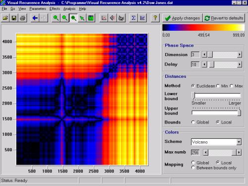
Here is an example of a recurrence plot constructed from the
weekly closing prices of the Dow Industrial Average index (file
DowJones.dat included with VRA).
For the actual analysis and meaningful results, it is probably a good idea to use a stationary time series. Also, to make RP more meaningful, the color mapping should be meaningful, too. For example, “hot” colors (yellow, red, and orange) can be associated with small distances between the vectors, while “cold” colors (blue, black) may be used to show large distances. This way one can visualize and study the motion of the system trajectories and infer some characteristics of the dynamical system that generated the time series. Here is how the recurrence plot of the chaotic signal (Rossler attractor, file Rossler.dat included with VRA) looks like:
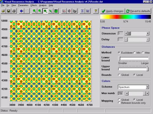
The global structure and local instability are the forces at work in the Rossler attractor, as can be seen from the recurrence plot above. Compare it with the recurrence plot of a strictly periodic signal (simple sine wave, file Sine.dat included with VRA):
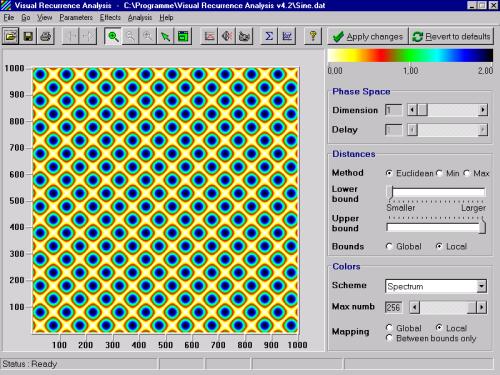
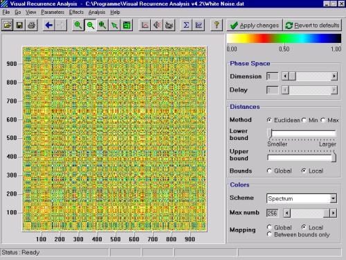
For random signals, the uniform (even) distribution of colors over the entire RP is expected. The more deterministic the signal is, the more structured the recurrence plot will be. Compare the recurrence plots above with that of the white noise time series (file WhiteNoise.dat included with VRA):
VISUAL RECURRENCE ANALYSIS HOME